squigualiser

squigualiser is a tool to Visualise nanopore raw signal-base alignment. signals (squiggles) + visualiser = squigualiser

Google Chrome is the recommended web browser to visualise these plots.

Watch the video to learn a few tricks to get the best out of the plots.

Squigualiser preprint - https://www.biorxiv.org/content/10.1101/2024.02.19.581111v2

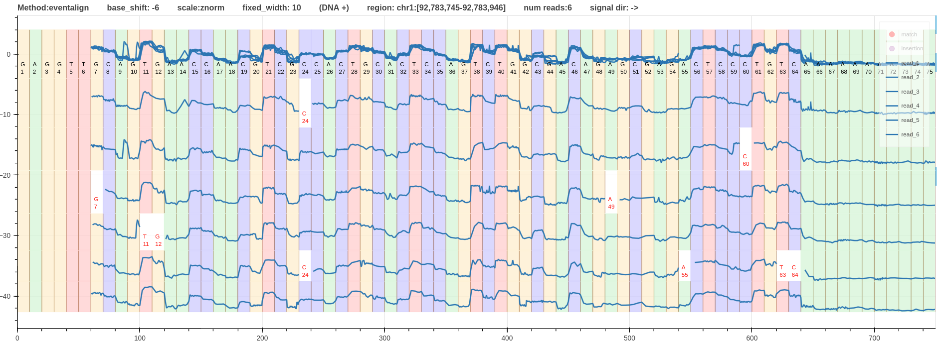
• Figure - A pileup view of DNA R10.4.1 signals that align to the region chr1:92,783,745-92,783,946.
• Click the link to open it on your browser.
• Go to Section Examples for more examples.

Table of Contents

1. Quickstart
2. Advanced Setup
3. Signal-to-read visualisation
   1. Option 1 - Using f5c resquiggle
   2. Option 2 - Using basecaller move table
   3. Option 3 - Using squigulator signal simulation
4. Signal-to-reference visualisation
   1. Option 1 - Using f5c eventalign
   2. Option 2 - Using basecaller move table
   3. Option 3 - Using squigulator signal simulation
5. Pileup view
6. Plot multiple tracks
7. BED annotations
8. Squigualiser GUI
9. Visualisation Enhancements
10. Base shift
11. Signal scaling
12. Plot conventions
13. Calculate alignment statistics
14. Notes
15. Examples

Quickstart

The easiest way to setup squigualiser would be to use precompiled binaries. Click on the arrow to expand the snippet of commands for your operating system.

For Linux distributions

wget https://github.com/hiruna72/squigualiser/releases/download/v0.6.1/squigualiser-v0.6.1-linux-x86-64-binaries.tar.gz -O squigualiser.tar.gz
tar xf squigualiser.tar.gz
cd squigualiser
./squigualiser --help

For macOS (Apple Silicon) distributions

curl -L https://github.com/hiruna72/squigualiser/releases/download/v0.3.0/squigualiser-v0.3.0-macos-arm64-binaries.tar.gz -O squigualiser.tar.gz
tar xf squigualiser.tar.gz
cd squigualiser
./squigualiser --help

For a quick test run the following:

wget https://hiruna72.github.io/squigualiser/docs/sample_dataset.tar.gz
# or use curl
curl -L https://hiruna72.github.io/squigualiser/docs/sample_dataset.tar.gz -o sample_dataset.tar.gz

tar xf sample_dataset.tar.gz
./squigualiser plot_pileup -f ref.fasta -s reads.blow5 -a eventalign.bam -o dir_out --region chr1:92,778,040-92,782,120 --tag_name "test_0"

export PATH=[path_to_squigualiser_dir]:$PATH to execute squigualiser from any location.

You can take a look at advanced setup below for instructions on installing using pip, conda or source.

Advanced setup

Click on the arrow to expand the relevant section.

Using python environment

python3.8 -m venv venv3
source venv3/bin/activate
pip install --upgrade pip
pip install squigualiser
squigualiser --help

Squigualiser has been tested with python 3.8.0, which should also work with anything higher. For installing relevant python versions, see the troubleshoot section below.

Using source code

git clone https://github.com/hiruna72/squigualiser.git
cd squigualiser
python3.8 -m venv venv3
source venv3/bin/activate
pip install --upgrade pip
pip install --upgrade setuptools wheel

export PYSLOW5_ZSTD=1 # if your slow5 file uses zstd compression and you have zstd installed, set
python setup.py install
squigualiser --help

Using conda environment

git clone https://github.com/hiruna72/squigualiser.git
cd squigualiser
conda create -n squig python=3.8.0 -y
conda activate squig

export PYSLOW5_ZSTD=1 # if your slow5 file uses zstd compression and you have zstd installed, set

python setup.py install
squigualiser --help

Troubleshoot: python versions

You can check your Python version by invoking python3 --version. If your native python3 meets this requirement of >=3.8, you can use that, or use a specific version installed with deadsnakes below. If you install with deadsnakes, you will need to call that specific python, such as python3.8 or python3.9, in all the following commands until you create a virtual environment with venv. Then once activated, you can just use python3. To install a specific version of python, the deadsnakes ppa is a good place to start:

# This is an example for installing python3.8
# you can then call that specific python version
# > python3.8 -m pip --version
sudo add-apt-repository ppa:deadsnakes/ppa
sudo apt-get update
sudo apt install python3.8 python3.8-dev python3.8-venv

Troubleshoot: Install zlib development libraries (and optionally zstd development libraries)

The commands to zlib development libraries on some popular distributions :

    On Debian/Ubuntu : sudo apt-get install zlib1g-dev
    On Fedora/CentOS : sudo dnf/yum install zlib-devel
    On OS X : brew install zlib

SLOW5 files compressed with zstd offer smaller file size and better performance compared to the default zlib. However, zlib runtime library is available by default on almost all distributions unlike zstd and thus files compressed with zlib will be more ‘portable’. Enabling optional zstd support, requires zstd 1.3 or higher development libraries installed on your system:

    On Debian/Ubuntu : sudo apt-get install libzstd1-dev # libzstd-dev on newer distributions if libzstd1-dev is unavailable
    On Fedora/CentOS : sudo yum libzstd-devel
    On OS X : brew install zstd

Signal-to-read visualisation

This section explains how you can use squigualiser to visualise a raw signal alignment against its basecalled read. Click on the arrow to expand the revalent method.

Option 1 - f5c resquiggle

Steps for using f5c resquiggle signal-to-read alignment

1. Install f5c v1.3 or higher as explained in f5c documentation.

2. Run f5c resquiggle

FASTQ=reads.fastq
SIGNAL_FILE=reads.blow5
ALIGNMENT=resquiggle.paf

f5c resquiggle -c ${FASTQ} ${SIGNAL_FILE} -o ${ALIGNMENT}

• Refer Note(2) for more information about --kmer-model [KMER_MODEL], which is optional.
• Refer Note(3) for more information about RNA.

1. Plot signal-to-read alignment

OUTPUT_DIR=output_dir
squigualiser plot -f ${FASTQ} -s ${SIGNAL_FILE} -a ${ALIGNMENT} -o ${OUTPUT_DIR} # to plot a selected read ID, you can provide -r 'READ_ID'.

Option 2 - basecaller move table

steps for using move table generated by the basecaller

1. Run basecaller (slow5-dorado, buttery-eel or ont-Guppy)

# buttery-eel (tested with v0.2.2)
buttery-eel -g [GUPPY exe path] --config [DNA model] -i [INPUT] -o [OUTPUT] --port 5558 --use_tcp -x "cuda:all" --moves_out
e.g buttery-eel -g [GUPPY exe path] --config dna_r10.4.1_e8.2_400bps_sup.cfg -i input_reads.blow5 -o basecalls.sam --port 5558 --use_tcp -x "cuda:all" --moves_out

# slow5-dorado (tested with v0.2.1)
slow5-dorado basecaller [DNA model] [INPUT] --emit-moves > [OUTPUT]
e.g. slow5-dorado basecaller dna_r10.4.1_e8.2_400bps_sup@v4.0.0 input_reads.blow5 --emit-moves > basecalls.sam

# ont-guppy (tested with v6.3.7)
guppy_basecaller -c [DNA model] -i [INPUT] --moves_out --bam_out --save_path [OUTPUT]
samtools merge pass/*.bam -o basecalls.bam # merge passed BAM files to create a single BAM file

1. Reformat move table (more info about reform).

# PAF output for plotting
ALIGNMENT=reform_output.paf
squigualiser reform --sig_move_offset 0 --kmer_length 1 -c --bam basecalls.sam -o ${ALIGNMENT}

• Refer Note(4) for more information on the PAF output.
• Refer Note(5) for a description about sig_move_offset.
• Refer Note(6) for handling a potential SAM/BAM error.

1. Plot signal-to-read alignment

FASTA_FILE=read.fasta
SIGNAL_FILE=read.blow5
OUTPUT_DIR=output_dir

# use samtools fasta command to create .fasta file from SAM/BAM file
samtools fasta basecalls.sam > ${FASTA_FILE}
# plot
squigualiser plot --file ${FASTA_FILE} --slow5 ${SIGNAL_FILE} --alignment ${ALIGNMENT} --output_dir ${OUTPUT_DIR}

Option 3 - Squigulator signal simulation

Steps for using Squigulator signal simulation software

1. Setup squigulator v0.2.1 or higher as explained in the documentation.

2. Simulate a signal (remember to provide -q and -c options).

REF=ref.fasta          #reference
READ=sim.fasta         #simulated reads
ALIGNMENT=sim.paf      #contains signal-to-read alignment
SIGNAL_FILE=sim.blow5  #simultated raw signal data

squigulator -x dna-r10-prom ${REF} -n 1 -o ${SIGNAL_FILE} -q ${READ} -c ${ALIGNMENT} # instead of dna-r10-prom, you can specify any other profile

1. Plot signal-to-read alignment.

OUTPUT_DIR=output_dir
squigualiser plot -f ${READ} -s ${SIGNAL_FILE} -a ${ALIGNMENT} -o ${OUTPUT_DIR} # to plot a selected read ID, you can provide -r 'READ_ID'.

Signal-to-reference visualisation

This section explains how you can use squigualiser to visualise a raw signal alignment against a reference. Click on the arrow to expand the relevant method.

Option 1: f5c eventalign

Steps for using f5c eventalign

1. Install f5c v1.3 or higher as explained in f5c documentation.
2. Align reads to reference genome

REF=genome.fa #reference
MAP_BAM=mapped.bam
FASTQ=read.fastq
samtools fastq basecalls.sam > ${FASTQ} # if basecalls are in sam format

# For DNA
minimap2 -ax map-ont ${REF} ${FASTQ} -t8 --secondary=no | samtools sort - -o ${MAP_BAM} && samtools index ${MAP_BAM} 

# For RNA (reference must be the transcriptome)
minimap2 -ax splice -uf -k14 ${REF} ${FASTQ} -t8 --secondary=no | samtools sort - -o ${MAP_BAM} && samtools index ${MAP_BAM} 

1. create f5c index

SIGNAL=reads.blow5
f5c index ${FASTQ} --slow5 ${SIGNAL}

1. f5c eventalign

ALIGNMENT=eventalign.bam
f5c eventalign -b ${MAP_BAM} -r ${FASTQ} -g ${REF} --slow5 ${SIGNAL} -a -o eventalign.sam
samtools sort eventalign.sam -o ${ALIGNMENT}
samtools index ${ALIGNMENT}

1. Plot signal to reference alignment.

OUTPUT_DIR=output_dir
REGION=chr1:6811404-6811443
squigualiser plot -f ${REF} -s ${SIGNAL_FILE} -a ${ALIGNMENT} -o ${OUTPUT_DIR} --region ${REGION} --tag_name "eventalgin"

Option 2 - basecaller move table

Steps for using move table generated by the basecaller

1. Run basecaller (slow5-dorado, buttery-eel or ont-Guppy)

# buttery-eel (tested with v0.2.2)
buttery-eel -g [GUPPY exe path] --config [DNA model] -i [INPUT] -o [OUTPUT] --port 5558 --use_tcp -x "cuda:all" --moves_out
e.g buttery-eel -g [GUPPY exe path] --config dna_r10.4.1_e8.2_400bps_sup.cfg -i input_reads.blow5 -o basecalls.sam --port 5558 --use_tcp -x "cuda:all" --moves_out

# slow5-dorado (tested with v0.2.1)
slow5-dorado basecaller [DNA model] [INPUT] --emit-moves > [OUTPUT]
e.g. slow5-dorado basecaller dna_r10.4.1_e8.2_400bps_sup@v4.0.0 input_reads.blow5 --emit-moves > basecalls.sam

# ont-guppy (tested with v6.3.7)
guppy_basecaller -c [DNA model] -i [INPUT] --moves_out --bam_out --save_path [OUTPUT]
samtools merge pass/*.bam -o basecalls.bam # merge passed BAM files to create a single BAM file

1. Reformat move table (more info on reform).

# PAF output for plotting
REFORMAT_PAF=reform_output.paf
squigualiser reform --sig_move_offset 0 --kmer_length 1 -c --bam basecalls.sam -o ${REFORMAT_PAF}

• Refer Note(4) for more information on the paf output.
• Refer Note(5) for a description about sig_move_offset.
• Refer Note(6) for handling a potential SAM/BAM error.

1. Align reads to reference genome

REF=genome.fa #reference
MAPP_SAM=map_output.sam

# For DNA
samtools fastq basecalls.sam | minimap2 -ax map-ont ${REF} -t8 --secondary=no -o ${MAPP_SAM} -

# For RNA (the reference must be the transcriptome)
samtools fastq basecalls.sam | minimap2 -ax splice -uf -k14 ${REF} -t8 --secondary=no -o ${MAPP_SAM} -

1. Realign reformatted move table to reference (more info on realign).

REALIGN_BAM=realign_output.bam
squigualiser realign --bam ${MAPP_SAM} --paf ${REFORMAT_PAF} -o ${REALIGN_BAM}

1. Plot signal-to-reference alignment

REGION=chr1:6811404-6811443
SIGNAL_FILE=read.blow5
OUTPUT_DIR=output_dir

# plot
squigualiser plot --file ${REF} --slow5 ${SIGNAL_FILE} --alignment ${REALIGN_BAM} --output_dir ${OUTPUT_DIR} --region ${REGION} --tag_name "optionA"

Option 3 - Squigulator signal simulation

Steps for using the signal simulation software (SAM output, recommended)

1. Setup squigulator v0.2.1 or higher as explained in the documentation.

2. Simulate a signal (remember to provide -a).

   REF=ref.fasta #reference
   READ=sim.fasta
   ALIGNMENT=sorted_sim.bam
   SIGNAL_FILE=sim.blow5
   NUM_READS=50 #number of reads to simulate
   squigulator -x dna-r10-prom ${REF} -o ${SIGNAL_FILE} -a sim.sam -n ${NUM_READS} && samtools sort sim.sam -o ${ALIGNMENT} && samtools index ${ALIGNMENT}
   

3. Plot signal-to-reference alignment.

   OUTPUT_DIR=output_dir
   REGION=chr1:6811404-6811443
   squigualiser plot -f ${REF} -s ${SIGNAL_FILE} -a ${ALIGNMENT} -o ${OUTPUT_DIR} --region ${REGION} --tag_name "optionB"
   

Steps for using the signal simulation software (PAF output)

1. Simulate a signal (remember to provide -c and –paf-ref).

REF=ref.fasta                 #reference
ALIGNMENT=sorted_sim.paf.gz   #sorted bgzip compressed PAF file containing signal to reference alignment
SIGNAL_FILE=sim.blow5         #simulated raw signals
NUM_READS=50                  #number of reads to simulate

For DNA
squigulator -x dna-r10-prom ${REF} -o ${SIGNAL_FILE} --paf-ref -c sim.paf -n ${NUM_READS}
sort -k6,6 -k8,8n sim.paf -o sorted_sim.paf
bgzip sorted_sim.paf
tabix -0 -b 8 -e 9 -s 6 ${ALIGNMENT}

For RNA
squigulator -x rna-r9-prom ${REF} -o ${SIGNAL_FILE} --paf-ref -c sim.paf -n ${NUM_READS}
sort -k6,6 -k9,9n sim.paf -o sorted_sim.paf
bgzip sorted_sim.paf
tabix -0 -b 9 -e 8 -s 6 ${ALIGNMENT}

Pileup view

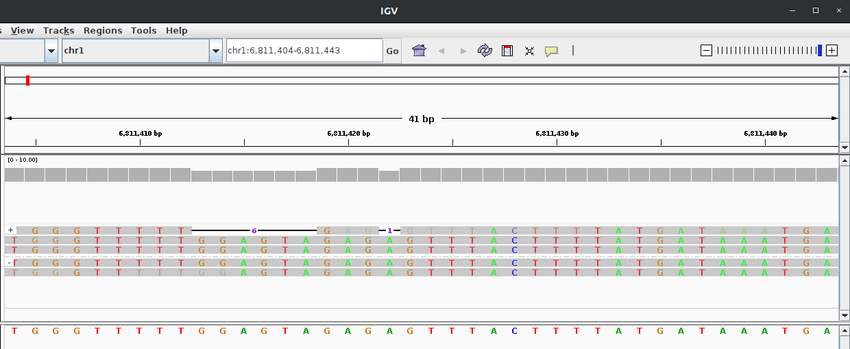
Similar to IGV pileup view now you can view the signal pileup view. To create a pileup view the following conditions should be met.

1. The plot is a signal-to-reference visualisation, not a signal-to-read.
2. A genomic region should be specified using the argument --region

First, create an alignment file by following the steps mentioned in Signal-to-reference visualisation

REGION=chr1:6811011-6811198
squigualiser plot_pileup -f ${REF} -s ${SIGNAL_FILE} -a ${ALIGNMENT} -o ${OUTPUT_DIR} --region ${REGION} --tag_name "pileup"

Here is an example DNA pileup plot created using the testcase 20.1. Here is an example RNA pileup plot created using the testcase 43.1.

Plot multiple tracks

For in depth analysis the user can visualize multiple pileup plots in the same web page.

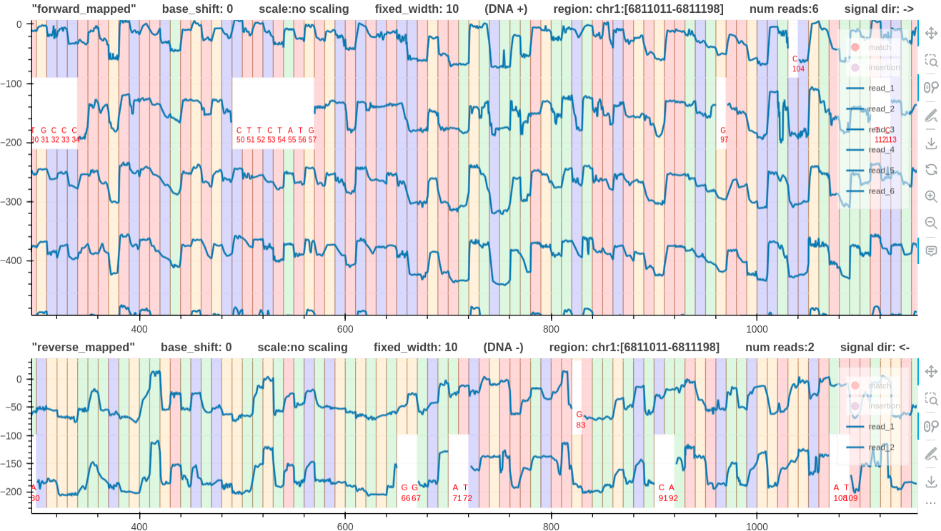
• The command plot_tracks only supports pileup views and takes a command_file.txt file as the input.
• The input file describes the number of commands, the dimension of each track, and the pileup commands.
• The following input command_file.txt file describes two pileup tracks with 900 and 200 heights for the first and second track respectively.
• Setting plot_heights=* in the command_file.txt or providing the argument --auto_height will automatically adjust the track height depending on the number of plots in each track.
• Note that the only difference between the two commands is that the second command has the additional --plot_reverse argument to plot reverse mapped reads. And -o or --output_dir argument is not necessary (ignored).

num_commands=2
plot_heights=900,200
squigualiser plot_pileup --region chr1:6,811,011-6,811,198 -f genome/hg38noAlt.fa -s reads.blow5 -a eventalign.bam --tag_name "forward_mapped"
squigualiser plot_pileup --region chr1:6,811,011-6,811,198 -f genome/hg38noAlt.fa -s reads.blow5 -a eventalign.bam --tag_name "reverse_mapped" --plot_reverse

Then use the plot_tracks command as below (remember to provide -o),

COMMAND_FILE="command_file.txt"
squigualiser plot_tracks --shared_x -f ${COMMAND_FILE} -o output_dir

Plot multiple tracks examples

1. Forward and reverse mapped reads in separate tracks link.
2. Different alignment methods (f5c eventalign and squigualiser’s realign) for RNA data in separate tracks link.
3. Real and simulated variants in separate tracks link.

BED annotations

Plots support BED file annotations. Use argument --bed [BED FILE] to provide the bed file to the plot command.

Here is an example RNA pileup plot created using the testcase 43.1 that supports bed annotations.

Squigualiser GUI

For GUI lovers, plots can be generated using a web application running on localhost (http://localhost:8000/home)

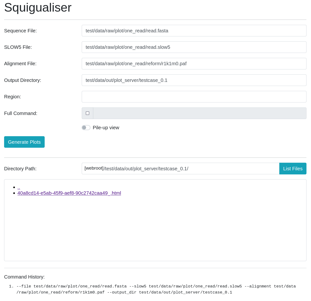
python src/server.py

Visualisation Enhancements

Base shift

User can shift the base sequence to the left by n number of bases by providing the argument --base_shift -n to plot and plot_pileup commands. This is helpful to correct the signal level to the base. A negative n value will shift the base sequence to the left. However, the user is adviced to use --profile (documented here) which automatically sets the --base_shift. For more information please refer base_shift and eventalignment and base_shift and reverse mapped reads.

Signal scaling

The commands plot and plot_pileup can take the argument --sig_scale. Provide the argument --sig_scale znorm to zscore normalize, --sig_scale medmad to median MAD normalize, and --sig_scale scaledpA to scale the raw signal to the pore model.

Plot Conventions

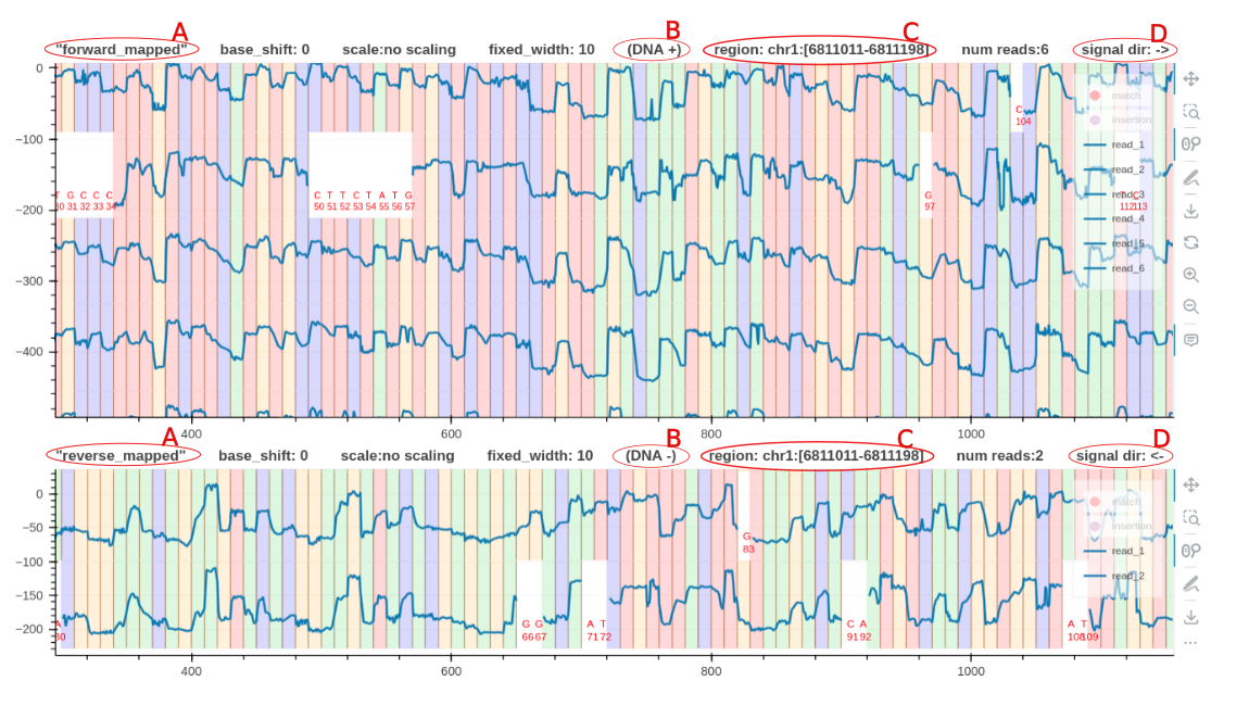
• A is a descriptive tag name to identify the plot.
• B indicates whether the positive or negative strand was used as the reference to align the signals. For RNA this will be RNA 3'->5'. Squigualiser only supports RNA reads mapped to the transcriptome.
• C always indicates the region using the positive strand coordinates, regardless of the forward and reverse mapped plots.
• D indicates the true sequencing direction of the signals.

Calculate alignment statistics

Calculate basic statistics of signal-to-read/reference alignments. Check here for the command. Check here for an example.

Notes

1. If your FASTQ file is a multi-line file (not to confuse with multi-read), then install seqtk and use seqtk seq -l0 in.fastq > out.fastq to convert multi-line FASTQ to 4-line FASTQ.
2. The optional argument --kmer-model KMER_MODEL can be used to specify a custom k-mer model if you wish.
3. To plot RNA signal-to-read alignment use the alignment file created using f5c resquiggle --rna -c ${FASTQ} ${SIGNAL_FILE} -o ${ALIGNMENT}. Also, provide the argument --rna to the visualising command. Currently, there exists no RNA kmer model for r10.4.1 chemistry.
4. The input alignment format accepted by squigualiser plot is explained here. This standard format made plotting a lot easier.
5. The argument sig_move_offset is the number of moves n to skip in the signal to correct the start of the alignment. This will not skip bases in the fastq sequence. For example, to align the first move with the first kmer --sig_move_offset 0 should be passed. To align from the second move onwards, --sig_move_offset 1 should be used.
6. Pysam does not allow reading SAM/BAM files without a @SQ line in the header. Hence, squigualiser reform script might error out with NotImplementedError: can not iterate over samfile without header. Add a fake @SQ header line with a zero length reference as follows,

   echo -e fake_reference'\t'0 > fake_reference.fa.fai
   samtools view out.sam -h -t fake_reference.fa.fai -o sq_added_out.sam
   

7. Squigulator’s signal simulation is a good way to understand the nature of the alignments. Please refer to the documentation about real_vs_simulated_signal.
8. For a explanation of the Guppy move table explanation see please refer here.

Examples

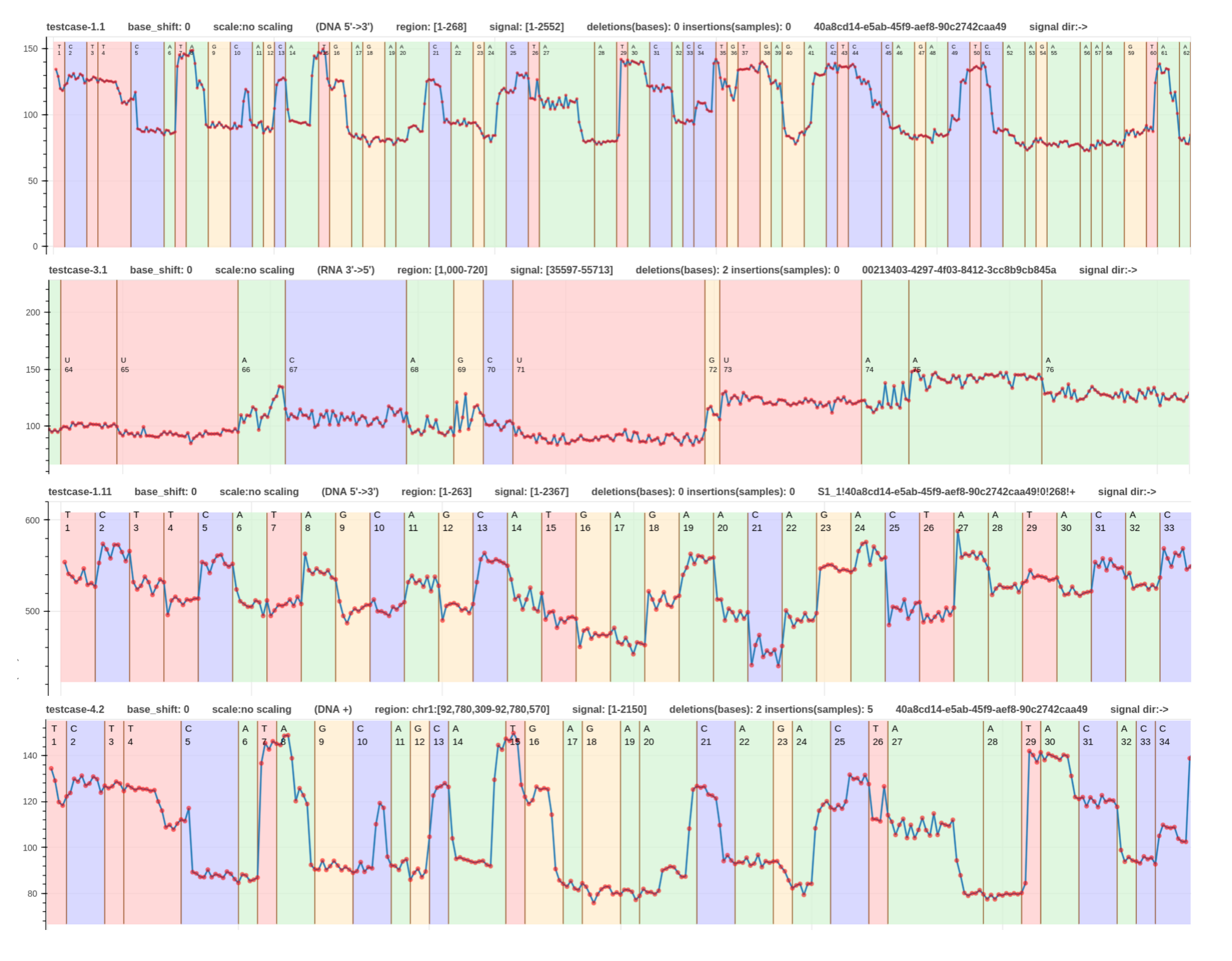
1. The first read is a signal-to-read alignment using guppy_v.6.3.7 move table annotation (link).
2. The second read is a signal-to-read alignment using f5c resquiggle output (link).
3. The third read is a signal-to-read alignment using the squigulator’s simulated output (link).
4. The fourth read (RNA) is a signal-to-read alignment using f5c resquiggle output (link).

• This signal-to-reference alignment aligns a signal to the region chr1:4270161-4271160.
• This is the same plot with a fixed base width.

These examples were generated using the testcases - 1.1, 2.1, 1.11, and 3.2 respectively in test_plot_signal_to_read.sh.

Please refer to the example pipelines to learn how to integrate squigualiser into your analysis.

Acknowledgement

Some code snippets have been taken from blue-crab, buttery-eel, readfish and bonito

This site is open source. Improve this page.